Optimization Algorithms are used to minimize or maximize an objective (loss) function. In the context of machine learning and optimization problems, we use them to iteratively adjust the parameters of a model to minimize a loss function and improve the model’s performance.
We know how backpropagation could be used to calculate the gradient of the loss function with respect to weights (parameter) in a neural network, but what methods can be applied to use this gradient to minimize loss?
There are perhaps hundreds of popular optimization algorithms, which can make it challenging to know which algorithm to use for a given optimization problem.
Let’s begin.
Overview
In this post, you will learn:
- What is an optimization algorithm in deep learning?
- Gradient Descent and its variants.
What is an Optimization Algorithm in Deep Learning?
Optimizers update the model in response to the output of the loss function.
Optimizers are a crucial element that fine-tunes a neural network’s parameters during training.
The primary goal is to minimize the calculated error or loss function.
In this post, you will learn gradient descent, which is the first-order algorithm that explicitly involves using the first derivative (gradient) to choose a direction to move in search space.
1- Gradient Descent
The input layer of a neural network receives input, and then the network produces outputs at an output layer. The network calculates the loss (error) for all samples at the output layer and backpropagates it to reduce the loss.
To train the weights to fit the task, and to minimize the loss, we need gradient descent.
In gradient descent, the goal is to find the global minimum of the loss function or a good local minimum with respect to weights when calculating the loss over the entire dataset. Here’s what it looks like:
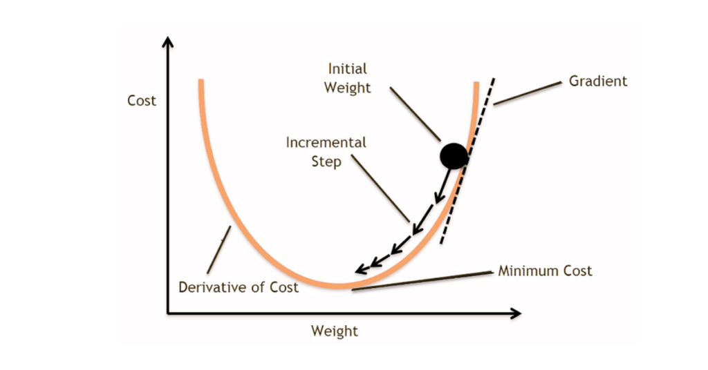
While mapping the loss vs weights, it may not be uniform, you may have a valley representing areas with low loss, and then small hills or peaks representing areas of higher loss followed by a valley. This uneven terrain can make the optimization process challenging.
Gradient descent comes into play by helping navigate this terrain. It works by calculating the slope (gradient) of the loss function w.r.t. each model parameter. The slope indicates the direction of steepest descent meaning, direction in which the loss decreases most rapidly.
But, how big of a step you can take?
The size of the step taken during each iteration is determined by the learning rate you set. It controls the magnitude of the parameter updates.
Gradient descent uses a constant learning rate. Additionally, it works well for convex functions.
Gradient descent works particularly well for convex functions as shown earlier. In convex optimization, the loss function has a single global minimum, meaning there is only one optimal solution.
What about Non-Convex Functions?
In deep learning, the loss functions are typically non-convex due to the highly complex non-linear nature of neural networks. Non-convex functions may have multiple local minima, saddle points, and plateaus, making optimization more challenging. Here’s what it looks like:
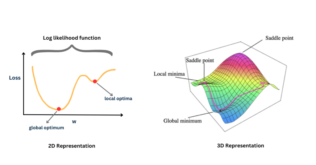
- Local Minimum: A point where the function has the lowest value within a small neighborhood of that pixel.
- Global Minimum: A point where the function has the lowest value across its entire domain.
- Saddle Point: A critical point of a function where the gradient is zero, but it is neither a local minimum nor a local maximum.
In non-convex optimization, local minima can trap optimization algorithms like gradient descent, preventing them from reaching the global minimum. Saddle points can also slow down convergence as the gradient is close to zero, but the point is not an optimum.
Additionally, gradient descent computes the gradient loss function w.r.t. model parameters using the entire dataset. This means that for each iteration in the optimization process, the algorithm considers every single training example to calculate the gradient. This is computationally expensive, especially in deep learning where larger datasets are employed.
Here are minor extensions to gradient descent that can overcome slow convergence, oscillations, or difficulty in setting an appropriate learning rate :
- Momentum
- Learning Rate Scheduling
- Adaptive Learning Rate Methods (AdaGrad, RMS Prop, Adam)
- Nesterov Accelerated Gradient
i. Momentum
Gradient Descent can oscillate in narrow valleys, slowing down convergence.
Momentum smoothens the optimization process by introducing a moving average of past gradients. This helps accelerate convergence, especially in the presence of noisy gradients or flat regions in the loss landscape. It allows the optimizer to build up momentum in directions where gradients consistently point, leading to faster convergence and more stable optimization paths.
ii. Learning Rate Scheduling
Choosing an appropriate learning rate is crucial as it affects the convergence speed and stability of the process.
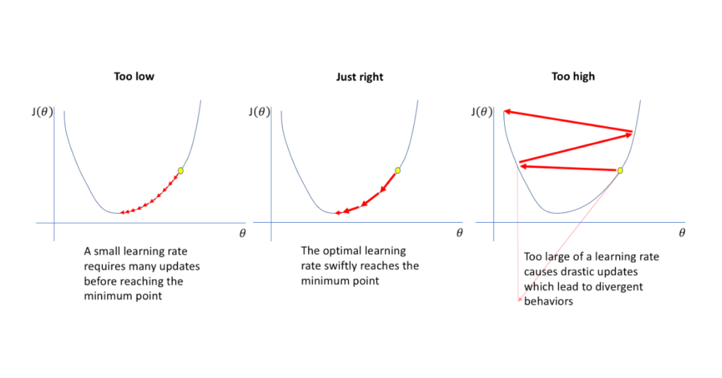
Here’s another figure that demonstrates the impact of learning rate on convergence.
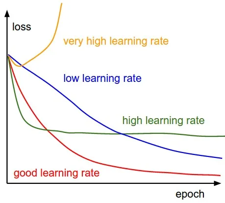
Learning rate scheduling adjusts the learning rate during training training based on certain criteria. Common strategies include decreasing the learning rate over time (e.g., exponential decay, step decay), or adapting the learning rate based on the behavior of the optimization process (e.g., AdaGrad, RMS prop, Adam).
These techniques help improve convergence and stability by making sure that the optimizer does not overshoot or get stuck in suboptimal solutions.
iii. Adaptive Learning Rate Methods (AdaGrad, RMS Prop, Adam)
Gradient descent uses a constant learning rate, this may not be optimal for all parameters and may lead to slow convergence.
Adaptive learning rate methods dynamically adjust the learning rate for each parameter based on their past gradient.
AdaGrad (Adaptive Gradient) Optimization Algorithm
Adapts learning rate based on the historical gradients for each parameter, giving smaller updates to parameters that have large gradients and vice versa. It maintains a separate learning rate for each parameter.
Adagrad is effective for sparse data and features because it automatically scales the learning rate based on the magnitude of gradients. This means that parameters with infrequent updates receive larger updates, while parameters with frequent updates receive smaller updates.
This helps in overcoming the issue of exploding or vanishing gradients in deep neural networks.
However, learning rate of Adagrad decays over time, which may result in very small learning rates in later stages of training. This may lead to premature convergence and difficulties in further learning.
Additionally, Adagrad accumulates squared gradients in the denominator, which can cause the learning rate to become too small, making it difficult for the model to escape from the saddle point.
RMSprop (Root Mean Square Propagation) Optimization Algorithm
RMSprop is an extension of AdaGrad that addresses its limitations by using a moving average of squared gradients to normalize the learning rate.
Instead of accumulating all past squared gradients, RMSprop calculates a moving average of squared gradients using exponential decay. This restricts the learning rate from decreasing too rapidly over time.
To help mitigate Adagrad’s issue of decaying learning rates, RMSprop normalizes the learning rate with root mean squares of the gradients. This allows RMSprop to better adapt to the varying magnitudes of gradients across different parameters.
However, RMSprop suffers from issues such as a decaying learning rate and difficulties in escaping saddle points.
Adam (Adaptive Moment Estimation) Optimization Algorithm
Adam combines the advantages of both momentum optimization and RMSprop. It calculates an exponentially decaying average of past gradients (like momentum) and an exponentially decaying average of past squared gradients (like RMSprop). These averages are then used to update the parameters with a learning rate that is adaptively scaled based on both the first and second moments of the gradient.
Compared to traditional optimizers with fixed learning rates, Adam is less sensitive to hyperparameters. It can perform well across a wide range of learning rates and other hyperparameters, reducing the need for extensive hyperparameter tuning.
By scaling the learning rates based on the magnitude of the gradients, Adam can navigate through narrow valleys and sharp turns without getting stuck or oscillating. This makes it more resilient to loss landscape curvature.
iv. Nesterov Accelerated Gradient (NAG) Optimization Algorithm
Nesterov Accelerated Gradient modifies the momentum update by taking into account the gradient ahead of its current position. This allows the optimizer to anticipate its next position and adjust its momentum accordingly, improving convergence speed.
This is especially useful in scenarios with noisy gradients.
Even though Adam is a powerful optimization algorithm that combines learning rates and momentum, NAG offers some unique advantages that complement the capabilities of Adam:
- NAG has a lookahead mechanism that helps it to anticipate the future position based on the current momentum, this helps it to navigate through regions of high curvature more efficiently.
- The lookahead step in NAG helps in adjusting the momentum before computing the gradient. This allows NAG to make smoother updates to the parameters, leading to more stable optimization paths.
- In cases with high curvature or narrow valleys in the loss landscape, NAG converges faster than Adam.
2 - Stochastic Gradient Descent (SGD)
In Stochastic Gradient Descent (SGD), the gradient of the loss function is computed using only one training example at a time. This means, that for a single iteration of the optimization process, a single training example is randomly selected from the dataset, and the gradient of loss function with respect to the model parameter is computed. The model parameters are then updated using this computed gradient.
SGD is computationally efficient, for large-scale datasets, as it requires computing gradient for one training example at a time. It
introduces stochasticity into the optimization process, which can help escape local minima and navigate through regions of high curvature in the loss landscape. SGD leads to faster updates and better generalization.
However, SGD can give noisy updates, leading to slower convergence. It requires more iterations as each update is based on only one training example at a time.
3 - Mini-Batch Gradient Descent
Instead of using the entire dataset (batch) or just one example (SGD) to compute the gradient. Mini-batch gradient descent computes the gradient using a smaller subset of training data, typically ranging from tens to hundreds of examples of ‘mini-batch’.
The model parameters are updated based on the gradient computed from this mini-batch.
Mini-batch gradient descent is computationally efficient as it processes multiple training examples simultaneously while introducing stochasticity. Provides faster convergence and better generalization compared to batch gradient descent and SGD.
However, the mini-batch may still exhibit some degree of noise and variance, depending on the size of the mini-batch and the dataset.
Summary
- In deep learning, optimization algorithms are crucial for updating a model’s parameters to minimize the loss function. This ultimately improves the model’s performance.
- Gradient descent finds the local minimum or global minimum. While gradient descent is effective for convex functions. It faces challenges with non-convex functions such as local minima, saddle points, and plateaus.
- Extensions of gradient descent have been developed, including momentum, learning rate scheduling, and adaptive learning rate methods to make optimization more efficient and robust.
- Stochastic gradient descent and Mini-batch gradient descent are variations of gradient descent that introduce stochasticity based on small subsets of training examples.
Related Articles
- How to Train a Neural Network with Multiple Parameters
- How to Understand and Implement Neural Networks: A Step-by-Step Guide
Further Readings
Related Videos
- What are Optimizers in deep learning? (Keras & TensorFlow) - Digital Sreeni
- Optimization for Deep Learning (Momentum, RMSprop, AdaGrad, Adam) - DeepBean
- Types of Optimization Algorithms - Maxwell Libbrecht

