Various milestones have marked the evolution of Artificial Intelligence (AI), from the early days of Symbolic AI to the emergence of Deep Learning. This post explores the historical context, challenges faced by early AI, and the transformative breakthroughs that led to the prominence of Deep Learning.
In this post, you will be provided with essential context around artificial intelligence, machine learning, and deep learning.
Overview
1- Artificial Intelligence
Before we begin, we need to understand what we’re talking about when we mention AI. What are artificial intelligence, machine learning, and deep learning? Are they even related to each other? If so, how?
In the 1950s, a handful of pioneers in the field of computer science coined the term Artificial Intelligence (AI) while pondering whether computers could be capable of THINKING. They came up with a definition of the field:
Interestingly, programmers introduced an approach called “Symbolic AI” for games like chess, involving hardcoded rules, and believed it to be machine learning within the field of AI.
i. What is Symbolic AI?
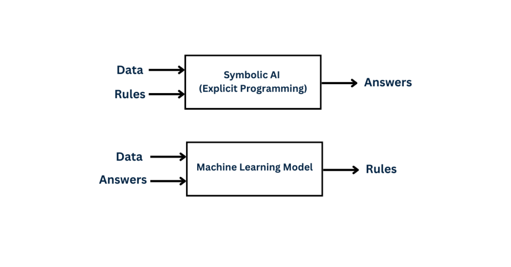
Humans input rules and data, process them according to the rules, and receive answers as output.
How Did Symbolic AI Became so Popular?
They believed that achieving human-level intelligence could involve handcrafting an explicitly large set of explicit rules for manipulating knowledge. Symbolic AI became a dominant paradigm from the 1950s to the 1980s and reached its peak during the expert system boom in the 1980s.
Drawbacks of Symbolic AI – Emergence of Machine Learning
It was then that pioneers came to realize that symbolic AI may have proved to be suitable for logical programs – playing chess. However, these explicit rules were not very effective in solving more complex fuzzy problems. These include image classification, speech recognition, and language translation. Thus, a new approach arose to take things to the next level – Machine Learning!
ii. Brief History of Machine Learning
Lady Ada Lovelace, a friend and collaborator of Charles Babbage, initiated it all by remarking on Charles’s invention Analytical Engine. The aim of the analytical engine was to use mechanical operations for automating computations in the field of mathematical analysis.
In 1843, Lady Ada Lovelace remarked that the analytical engine could do whatever we know how to order it to perform, meaning, it has no pretensions to originate anything.
AI pioneer Alan Turing later quoted this remark in his landmark 1950 paper, which included a Turing test and key concepts that would shape the field of AI. Alan pondered whether computers have the capability of learning and originality, and he concluded that they actually could.
So how did Machine learning arise? From the very question that originated from Ada Lovelace’s remarks: could a computer go beyond “what we know how to order it to perform” and learn on its own how to perform a specific task? Could a computer surprise us? Could it learn the rules automatically, without being explicitly programmed?
iv. Symbolic AI Vs. Machine Learning
Humans input data as well as the expected answers into Machine Learning, and the output comprises the rules generated by the data. But how is this useful? The rules generated from the data and expected outputs can be applied to new data, resulting in original answers—Bam!

The ML system learns instead of being programmed with hardcoded rules. In this process, the model encounters relevant examples and utilizes them to identify statistical structures, enabling the generation of rules for automating the task. Here’s an example:
Imagine you have a bulk of vacation pictures that you took this summer. Now you want to tag these pictures to keep a memory of places you’ve been to and things you saw. You take vacations every year, and it is not feasible to tag each picture each year by yourself, right?
To make the task easier, you could present tagged pictures to the machine learning system. The system would learn statistical rules associating specific pictures to specific tags. Once it has been trained, you can use it every year to tag pictures.
One thing to remember: Machine learning is tightly related to mathematical statistics. Unlike statistics, ML deals with large, complex datasets – millions of images with thousands of pixels for each image.
Now that we know what machine learning is and how it emerged. Before we dive into the subfield of machine learning - “Deep Learning”, let’s go through some classical machine learning approaches.
iii. Probabilistic Modeling
Dated back to the 17th century, one of the earliest forms of machine learning is probabilistic modeling, an application of principles of statistics to data analysis. It involves representing uncertain quantities as probability distributions. It also provides a framework for reasoning about uncertainty and making predictions based on probabilistic assumptions.
Simply put, it involves using probability theory to model and make predictions or decisions in the presence of incomplete or noisy information. Here are the key components:
- Random variables – These are variables whose values are uncertain, and used to represent features or parameters of interest.
- Probability Distributions – These describe the likelihood of different values that a random variable can take, it can be either discrete or continuous.
- Parameters – These characterize the underlying distribution. These parameters are estimated from available data.
Example – Use a probabilistic model to perform image segmentation.
- Random Variables – In a colored image, random variables can be color values of each pixel, characterized by three random variables corresponding to (Red, Green, and Blue) color channels. Each color follows a continuous distribution.
- Probability Distribution – In the colored image, the probability distribution is the likelihood of different color values that a random pixel can take. This can be modeled using probability distributions, such as Gaussian distribution, for each channel. For instance, model the red channel as a Gaussian distribution with mean and standard deviation and do the same for green and blue channels. Then model the joint distribution of RGB values as a multivariate Gaussian distribution.
- Parameters – In this context, the mean and standard deviation would be the parameters.
Application:
The trained probabilistic model calculates the likelihood of observing a specific color at each pixel. This information can be used in algorithms like Expectation Maximization (EM) to make decisions about the presence of objects or boundaries in the image.
iv. Early Neural Networks
Refers to the initial developments and applications of artificial neural networks (ANNs) in the field of AI. Inspired by the structure and functioning of the human brain, neural networks laid the foundation of ANNs. Let’s go through some key milestones and characteristics of neural networks:
- McCulloch-Pitts Neuron Model – The earliest model of an artificial neuron, proposed by Warren McCulloch and Walter Pitts in 1943. This laid the foundation for the development of artificial neural networks.
- Perceptron – Designed for binary classification tasks by Frank Rosenbolt, in 1957 based on McCulloch-Pitts neuron model, perceptrons could learn to make decisions by adjusting their weights based on errors in predictions. However, their learning capability was limited as they could only learn linearly separable functions. This resulted in struggles with tasks requiring non-linear decision boundaries.
- Backpropagation Algorithms – To overcome the limitation of single-layer perceptron, backpropagation algorithms were introduced in 1970s-1980s. This allowed for the training of networks with multiple layers.
- Multi-Layer Perceptrons – With the addition of hidden layers in the 1980s, the networks became able to learn complex, non-linear mappings from input to output.
- Hinton’s Boltzmann Machines – Introduced by Geoffery Hinton in 1985, it is a type of stochastic neural network that uses a probabilistic approach to learning.
- Recurrent Neural Networks (RNNs) and Long Short-Term Memory (LSTM) – In the late 1980s and 1990s, to deal with sequential data, RNNs and LSTMs were introduced. Moreover, these models were also able to capture dependency over time.
Despite these advancements, early neural networks faced challenges such as limited computational resources, lack of large datasets, and vanishing gradient problem. Despite the challenges, this foundational work laid the groundwork for the rapid advancement of neural network research and applications.
v. Kernel Methods
As neural networks started to gain some respect and attention among researchers in the 1990s, a new approach to machine learning arose to fame: kernel methods. A group of classification algorithms, particularly powerful for solving complex, non-linear problems such as classification, regression, and dimensionality reduction.
The central idea is to implicitly map input data to a high-dimensional feature space, where one can exploit linear relationships in that space to solve non-linear problems in the original input space.
- Kernel Function – It computes similarity between pairs of data points in input space allowing the algorithm to work in a high-dimensional space without explicitly calculating the transformations.
- Feature Space Mapping – Allows implicitly mapping data into high-dimensional feature space. This mapping is non-linear which allows the algorithm to capture complex relationships between data points.
- Kernel Trick – It computes the dot product of data points in feature space directly in the input space, making computations more efficient.
- Support Vector Machines (SVM) – A popular class of algorithm that uses kernel methods. SVMs find a hyperplane in high-dimensional space that maximally separates different classes or predicts continuous target variables.
Various domains widely use kernel methods due to their flexibility in handling non-linear relationships. It is worth noting that the choice of kernel and its parameters can have a significant impact on the performance of the algorithm.
vi. Decision Tree, Random Forest, and Gradient Boosting Machines
Let’s start with decision trees, these are flow-chart-like structures that let us classify input data points or predict output values given inputs. These are easy to visualize and interpret. In the 2000s, attention gravitated towards Decision Trees, and by 2010, they often took preference over kernel methods. Here’s why:
- Decision trees (DTs) offer crucial interpretability in model understanding.
- The transparency of DTs is advantageous for explaining decisions in various domains, such as medical scenarios.
- The decision-making process in DTs is transparent, in contrast to kernel methods, often seen as black-box models due to high-dimensional mapping.
- DTs can be effectively regularized to prevent overfitting by adjusting parameters like maximum depth and minimum samples.
- Kernel methods may require additional regularization techniques to address overfitting concerns.
Random Forest algorithm, an ensemble of decision trees, trains each tree on a random subset of data and features. The final decision results from averaging or voting over predictions of individual trees. Moreover, known for providing feature importance scores, being robust to noisy data and outliers, and reducing overfitting, it quickly gained attention when the machine learning competition website Kaggle started in 2010.
This was until 2014, when gradient boosting machines took over. Much like random forest, this is a machine learning technique based on ensembling weak prediction models. Gradient boosting builds trees sequentially, with each tree correcting errors made by the previous ones. Considered one of the best algorithms for handling nonperceptual data, it is commonly employed in Kaggle competitions.
2- What Makes Deep Learning Different?
The primary reason that deep learning took off so quickly is that it makes problem-solving much easier. Traditional machine learning models often require manual feature engineering where experts design specific features that the model uses for learning.
Previous machine learning techniques (shallow learning) involved transforming data into one or two successive representation spaces, usually via simple transformations. Humans had to manually engineer good layers of representations for their data – feature engineering
In deep learning, the model automatically learns hierarchical representations of features from raw data. In deep learning, all features are learned in one pass rather than having to engineer them manually. This greatly simplified the machine learning workflows, often replacing multistage pipelines with a single, simple, end-to-end deep learning model.
If that’s the case, can we get the same benefits as deep learning by using shallow methods over and over again? Interestingly, that’s not the case, and here’s why:
- Diminishing Returns – If you keep applying shallow methods one after another, the improvement you get becomes smaller and smaller.
- Optimal First Layer – The optimal first representation layer in a three-layer model (like in deep learning) may not be the best first layer for a one or two-layer model (like in repeated shallow methods). This means that different model structures may require different starting points for optimal learning.
- Joint Feature Learning – Deep learning enables a model to learn all layers of representation simultaneously, a process known as joint feature learning. This approach empowers the model to acquire complex and abstract representations.
- Single Feedback Signal – A single feedback signal supervises everything in deep learning, guiding any changes in the model toward the ultimate goal.
Now that you know how deep learning took off and gained immense attention. It’s time to look at how we can implement deep learning. Here’s a post to kick-start your journey of understanding and implementing a neural network:
How to Understand and Implement Neural Networks: A Step-by-Step Guide
Summary
In this post, you learned:
- Historical content of Artificial Intelligence – pioneers exploring the possibility of computers thinking
- From symbolic Artificial Intelligence to Machine Learning – This allows computers to learn from data rather than explicit programming
- Brief history of Machine Learning – Lady Ada Lovelace’s remarks sparked the question of whether computers could go beyond predefined tasks.
- Classical Machine Learning Approaches – Probabilistic modeling to model uncertain quantities, early neural networks, kernel methods, decision trees, random forest, and gradient boosting machines
- What Makes Deep Learning Different – Automated hierarchical feature representation learning from raw data, eliminating the need for manual feature engineering, joint feature learning
Related Books
- Deep Learning, 2016
- Deep Learning with Python, 2021


