Best Activation Functions – Within the architecture of a neural network, the choice of activation functions between the hidden layer and output layer is crucial in determining the learning behavior and predictive capabilities of a neural network model. Therefore, a careful choice of these functions must be made for each deep learning neural network project.
Let’s get started.
Overview
In this post, you will learn:
- Activation functions.
- How to choose the best activation functions for the hidden layers.
- How to choose the best activation functions for the output layer.
1- Activation Function
The fundamental role of activation functions is to allow the neural networks to capture complex relationships within data.
The choice of activation functions has a significant impact on the capability and performance of the neural network.
A network has three types of layers, including an input layer that contains raw input from the domain, hidden layers that take input from one layer and pass output to the next layer, and output layers that make a prediction.
Now, let’s learn activation functions for hidden layers first:
2- Activation Functions for Hidden Layers
In a neural network, hidden perform intermediate computations between the input layer and the output layer. They’re responsible for transforming the input data in a way that allows the network to learn complex patterns and relationships.
Logistic regression classification algorithms widely utilize the sigmoid activation function, also recognized as the ‘logistic’ function.
To enable neural networks to learn complex data, non-linear activation functions are applied to neurons in the hidden layers. These functions allow the network to model intricate relationships that may not be captured by simple linear transformations.
Here are the most commonly used activation functions in hidden layers:
- Rectified Linear Activation (ReLU)
- Logistic (Sigmoid)
- Hyperbolic Tangent (tanh)
Now, let’s dive deeper into each of them.
i. Sigmoid Hidden Layer Activation Function
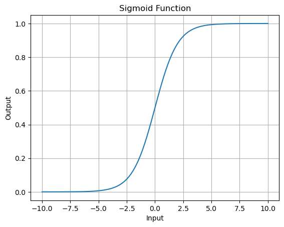
Logistic regression classification algorithms widely utilize the sigmoid activation function, also recognized as the ‘logistic’ function. It squashes real-valued input into a range between 0 and 1.
When the input is large and positive, the sigmoid function produces an output close to 1.0, indicating a high probability or confidence level. Conversely, when the input is large and negative, the sigmoid function produces an output close to 0.0 indicating a low probability or confidence level.
Mathematically, we calculate sigmoid activation function as follows:
\frac{1}{1+e^{-x}}
Here is a code snippet that calculates outputs for a range of values and creates a plot of inputs versus outputs:
import numpy as np
import matplotlib.pyplot as plt

def sigmoid(x):
    return 1 / (1 + np.exp(-x))

# Generate input values
x_values = np.linspace(-10, 10, 100)

# Calculate sigmoid function values
y_values = sigmoid(x_values)

# Plot sigmoid function
plt.plot(x_values, y_values)
plt.title('Sigmoid Function')
plt.xlabel('Input')
plt.ylabel('Output')
plt.grid(True)
plt.show()
Sigmoid is an S-shaped function, as you can see below:
When utilizing the sigmoid function in hidden layers, consider adopting the ‘Xavier Normal’ or ‘Xavier Uniform’ weight initialization. Moreover, the input data to the range 0-1, aligning with the activation function’s range can also improve both the model’s performance and stability.
ii. Tanh Hidden Layer Activation Function
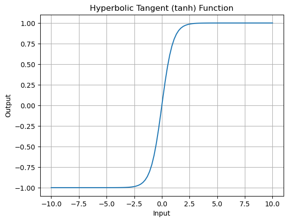
The hyperbolic tangent (tanh) activation function is a scaled and shifted version of the sigmoid function.
This function takes any real value as input and outputs values in the range -1 to 1. When the input is large and positive, the sigmoid function produces an output close to 1.0. When the input is large and negative, the sigmoid function produces an output close to -1.1 indicating a low probability or confidence level.
Mathematically, we calculate Tanh function as follows:
\text{tanh}(x) = \frac{\exp(x) - \exp(-x)}{\exp(x) + \exp(-x)}
In this formula:
- x represents input value
- exp(x) denotes the exponential function e^x, where e is Euler’s number.
Here is a code snippet that calculates outputs for a range of values and creates a plot of inputs versus outputs:
import numpy as np
import matplotlib.pyplot as plt

# Define the tanh function
def tanh(x):
    return np.tanh(x)

# Generate input values
x_values = np.linspace(-10, 10, 100)

# Calculate tanh function values
y_values = tanh(x_values)

# Plot tanh function
plt.plot(x_values, y_values)
plt.title('Hyperbolic Tangent (tanh) Function')
plt.xlabel('Input')
plt.ylabel('Output')
plt.grid(True)
plt.show()
Similar S-shape as the sigmoid function but Tanh is scaled and shifted version of sigmoid.
iii. ReLU Hidden Layer Activation Function
The rectified linear unit function or simple ReLU, is the most commonly used activation function within hidden layers.
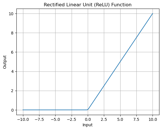
It is simple to implement and effective in overcoming the limitations of both sigmoid and tanh activation functions. It simply outputs the input value if it is positive, otherwise zero, making it highly efficient for both forward and backward propagation during training.
Other activation functions like sigmoid and tanh encounter the vanishing gradient problem, preventing the model from being trained. ReLU addresses this issue.
However, consistent negative inputs to a ReLU neuron may cause the neuron to output zero for all inputs and effectively ‘die out’.
Mathematically, we calculate ReLU activation function as follows:
where
f(x) = max (0,x)
- f(x) represents the output of the ReLU activation function for given input x .
- max is the maximum function, which outputs the larger of the two values provided as arguments.
- 0 is the threshold below which the output of the ReLU function is zero.
- x is the input to the ReLU function.
Here is an example code to visualize the ReLU activation function:
import numpy as np
import matplotlib.pyplot as plt

# Define the ReLU function
def relu(x):
    return np.maximum(0, x)

# Generate input values
x_values = np.linspace(-10, 10, 100)

# Calculate ReLU function values
y_values = relu(x_values)
# Plot ReLU function
plt.plot(x_values, y_values)
plt.title('Rectified Linear Unit (ReLU) Function')
plt.xlabel('Input')
plt.ylabel('Output')
plt.grid(True)
plt.show()
Here’s what it looks like:
Generally, It is a good practice to use ‘He Normal’ or ‘He Uniform’ weight initialization method. Scaling input data to a range of 0-1 (normalization) also helps in improving the stability and performance of the model.
3- Choosing the Best Activation Functions for Hidden Layers
In most cases, all hidden layers within a neural network will have the same activation function.
Imagine you’re building a team of workers (neurons) in a company (neural network). Each worker has a rule (activation function) to decide whether they should do their task or not. Having the same rules for all workers ensures consistency.
Using the same activation function in all hidden layers of the neural network ensures consistency in how information is processed and represented throughout the network.
Both the sigmoid and tanh functions can make the model more susceptible to problems during training by introducing the vanishing gradient problem.
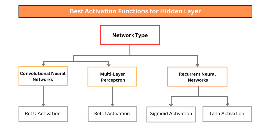
The choice of activation function is based on the network architecture you’re employing. Here’s a general guideline for selecting activation functions for different architectures:
- For Convolutional Neural Networks (CNNs) and Multilayer Perceptrons (MLPs), variants of ReLU activation functions are used due to their ability to handle sparse activations and alleviate vanishing gradient problem.
- For Recurrent Neural Networks, Tanh and sigmoid functions are used within their gates to control the flow of information over time.
Here’s a figure to summarize which activation functions to use based on the neural network architecture selected.
4- Activation Functions for Output Layer
Output layers help the neural network model to directly output a prediction.
The choice of the output layer depends on the task. However, here are the three most commonly used activation functions that you may want to consider:
- Logistic (Sigmoid)
- Linear
- Softmax
Let’s have a closer look at each one of them:
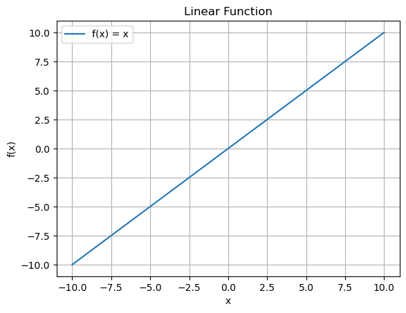
i. Linear Output Activation Function
In neural networks, the linear activation function, also known as the identity function, serves as one of the simplest activation functions.
The reason behind this is that the linear function does not change the weighted sum of the input in any way and returns the value directly.
Mathematically, we can calculate the linear activation function as follows:
f(x) = x
where:
x represents input to the neuron
f(x) represents the output to the neuron
import numpy as np
import matplotlib.pyplot as plt

# Define the linear function
def linear_function(x):
    return x

# Generate input values
x_values = np.linspace(-10, 10, 100)

# Calculate output values using the linear function
y_values = linear_function(x_values)

# Plot the linear function
plt.plot(x_values, y_values, label='f(x) = x')

# Add labels and title
plt.xlabel('x')
plt.ylabel('f(x)')
plt.title('Linear Function')
plt.grid(True)
plt.legend()

# Show plot
plt.show()
We can see a diagonal line shape:
ii. Sigmoid Output Activation Function
We have already discussed the sigmoid function earlier. Specifically for binary classification tasks, the sigmoid activation function is used in the context of the output layer. Let’s review the shape of this function once again

The sigmoid function squashes the output to the range [0,1], representing probabilities. This function
iii. Softmax Output Activation Function
Softmax is a mathematical function that converts a vector of numbers into a vector of probabilities.
This function outputs a vector of probabilities, where each element represents the likelihood of the corresponding class.
It is related to argmax function that outputs 0 for all options and 1 for chosen options. Softmax is a softer version of argmax as it considers relative magnitude of all values and produces a probability distribution that reflects their strengths. It’s as if each value gets a “soft vote” rather than a definitive win.
Mathematically, we can calculate Softmax activation function as follows:
\text{softmax}(x_i) = \frac{e^{x_i}}{\sum_{j=1}^{N} e^{x_j}}
where:
- e is Euler number, the base of the natural algorithm
- x_i is the score (logit) associated with class i
- The numerator computes the exponential of the score x_i
- The denominator computes the sum of exponentials for all scores in the vector x.
- Finally, each score x_i is divided by a sum of exponentials to normalize the probabilities, ensuring they sum up to 1.
Here’a a code example to demonstrate the softmax. function:
import numpy as np

def softmax(x):
    """Compute softmax values for each score in the input array."""
    exp_scores = np.exp(x)
    probabilities = exp_scores / np.sum(exp_scores, axis=0)
    return probabilities

# Example scores (logits)
scores = np.array([2.0, 1.0, 0.1])

# Compute softmax probabilities
softmax_probs = softmax(scores)

# Print original scores and softmax probabilities
print("Original Scores:", scores)
print("Softmax Probabilities:", softmax_probs)
Here’s the output
Original Scores: [2.  1.  0.1]
Softmax Probabilities: [0.65900114 0.24243297 0.09856589]
5- Choosing the Best Activation Functions for Output Layer
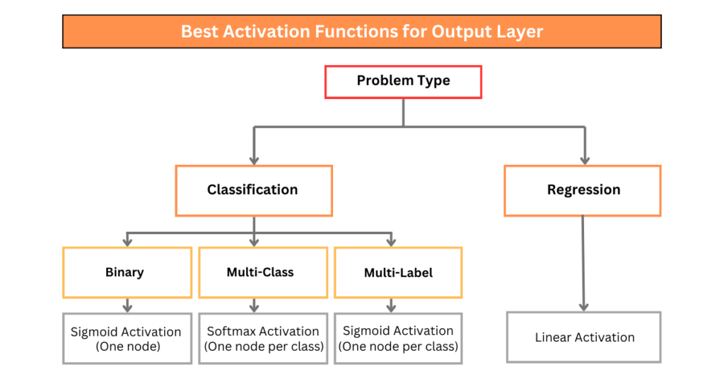
Choosing the activation function for the output layer solely depends upon the problem that you are solving.
We can divide the prediction problem into two main groups: predicting a categorical variable (classification) and predicting a numerical variable (regression).
i. Regression:
For predicting numerical variables, use a linear activation function.
Example: One node with linear activation
ii. Classification
For a classification problem, where the goal is to predict labels rather than numerical values, you can use either sigmoid or softmax, depending upon the classification problem you have.
- Binary Classification
If your problem has two mutually exclusive classes, you can use a sigmoid function. The sigmoid function squashes the output to a range between 0 and 1, representing the probability of belonging to one class.
Example: One node with sigmoid activation
- Multi-Class Classification
If your problem has more than two mutually exclusive classes, for instance, a digit recognition problem where you have 10 classes of digits (0-9) to predict, employ softmax activation function.
Softmax normalizes the output into a probability distribution over multiple classes, facilitating the prediction of probabilities for each class.
Example: One node per class with softmax activation
- Multi-Label Classification
When dealing with multiple mutually inclusive classes, each example belongs to one or more classes.
Use a sigmoid activation function for each class, allowing for independent binary classification of each class.
Example: One node per class with sigmoid function.
Here’s a figure that summarizes how to choose an activation function for the output layer of your network.
Summary
- Choosing the activation function depends upon the problem you are working on.
- Activation functions for hidden layers depend upon the network architecture you have, for CNNs and MLPs you can use ReLU activation, for RNNs, you can go with sigmoid and tanh activation functions.
- Activation functions for output layers depend upon the problem you are working on. For a regression problem, you can use linear activation function. For binary classification, you can use sigmoid activation, for multi-class classification, use softmax activation with each node, and for multi-label classification, use sigmoid for each output layer node.
Lastly,
We say activation functions are learning decision boundaries, but what do we mean by learning?
In the next article, you will learn how the machine learning model is trained to learn parameters (in case of a neural network with only one neuron with parameters such as weights and bias)


